Linear Regression
In the last unit you ran a complete machine learning workflow. You split data, trained a model, made predictions, and measured accuracy — all in about twenty lines of code. But there was a gap: you used a Decision Tree without understanding what it was doing.
This unit closes that gap for a different algorithm — Linear Regression. It’s the simplest predictive model in machine learning, and it’s the right place to start understanding what .fit() actually does.
The problem
Suppose you want to predict how much a house will sell for. You have data on past sales — the size of each house in square feet, and the price it sold for.
size_sqft | price
----------|--------
800       | 150000
1200      | 210000
1500      | 260000
2000      | 340000
2400      | 400000
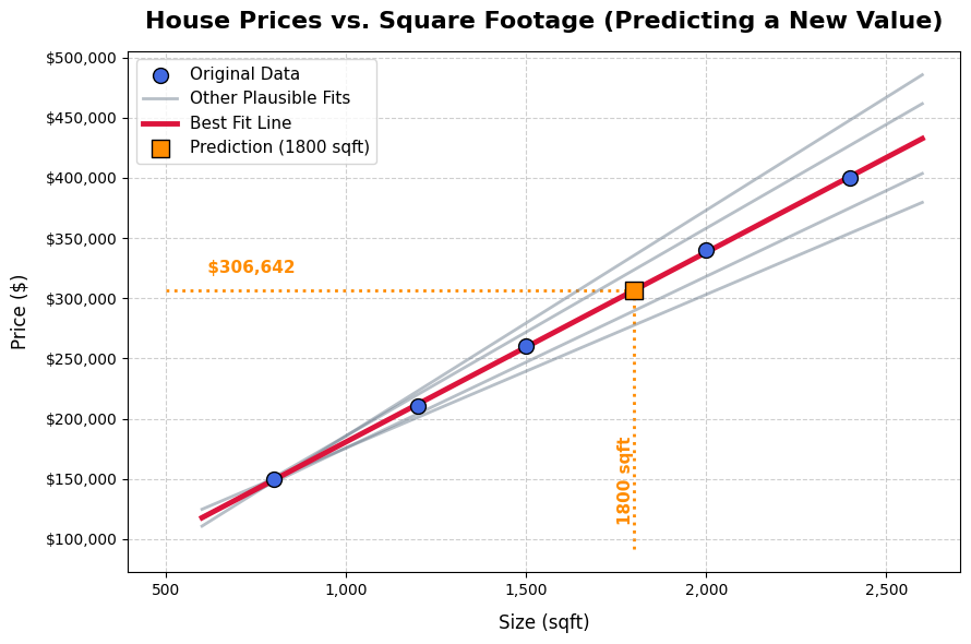
You could plot this data and draw a straight line through it. That line could then be used to predict the price of a house you’ve never seen before — just find its size on the x-axis, move up to the line, and read off the price.
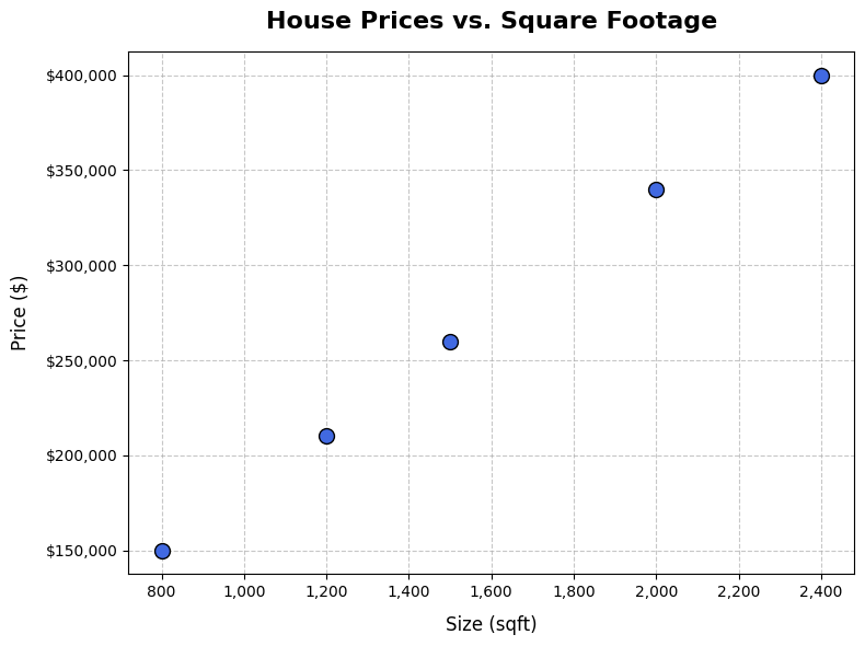
That is linear regression. The algorithm finds the best straight line through your data.
The equation of a line
You may have seen this from school:
y = mx + b
yis what you’re predicting (house price)xis your input (house size)mis the slope — how much y increases for every one-unit increase in xbis the intercept — the value of y when x is zero
In machine learning these are called weights and bias, or coefficients and intercept, but the idea is the same. The model is just a line.
When you call .fit(), the algorithm finds the values of m and b that make the line fit your training data as closely as possible.
What “best fit” means
There are many lines you could draw through a scatter of points. The question is which one is best.
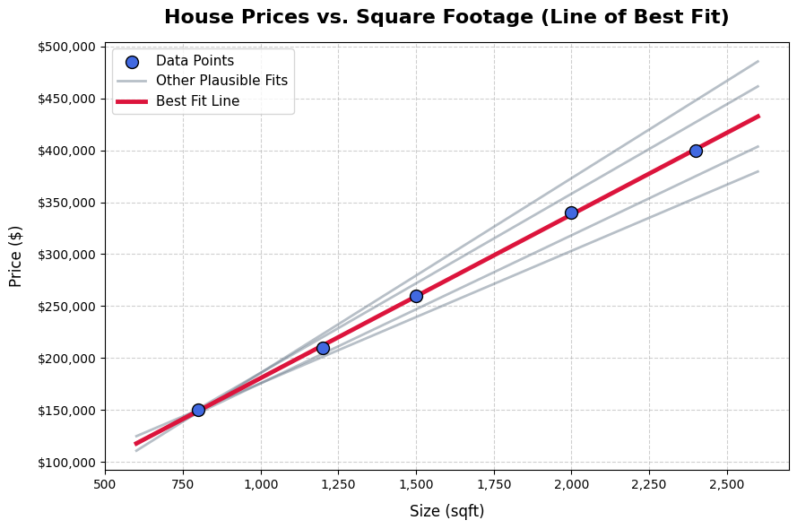
Linear regression measures “best” by looking at the error on each training example — the vertical distance between the actual data point and the line. These distances are called residuals.
The algorithm minimises the sum of those residuals squared. This is called Ordinary Least Squares — minimising the sum of squared errors. Squaring the distances does two things: it makes all errors positive (so they don’t cancel out), and it penalises large errors more than small ones.
The line that minimises this total squared error is the line of best fit.
You don’t need to do this calculation yourself. Scikit-learn handles it entirely when you call .fit(). But knowing what it’s doing explains why the line ends up where it does.
Linear regression in code
import pandas as pd
from sklearn.linear_model import LinearRegression
from sklearn.model_selection import train_test_split
from sklearn.metrics import mean_absolute_error

# Load data
df = pd.read_csv("houses.csv")
X = df[["size_sqft"]]
y = df["price"]

# Split
X_train, X_test, y_train, y_test = train_test_split(X, y, test_size=0.2, random_state=42)

# Train
model = LinearRegression()
model.fit(X_train, y_train)

# Predict
predictions = model.predict(X_test)

# Evaluate
mae = mean_absolute_error(y_test, predictions)
print(f"Mean Absolute Error: £{mae:,.0f}")
The structure is identical to the workflow you learned last unit. The only things that changed are the import (LinearRegression instead of DecisionTreeClassifier) and the evaluation metric.
A new evaluation metric: MAE
In the last unit you used accuracy — the percentage of correct predictions. That worked because the output was a category (passed or failed).
Linear regression predicts a number. There’s no “correct” or “incorrect” — only how close you were. That’s why you use a different metric.
Mean Absolute Error (MAE) is the average distance between your predictions and the actual values:
MAE = average of |actual - predicted| for all test examples
If your model predicts house prices with an MAE of £15,000, it means your predictions are off by £15,000 on average. Whether that’s acceptable depends on the context — it’s great for a £500,000 house and poor for a £60,000 flat.
MAE is easy to interpret because it’s in the same units as your target variable.
Inspecting the model
Once trained, you can look directly at what the model learned:
print(f"Slope:     {model.coef_[0]:,.2f}")
print(f"Intercept: {model.intercept_:,.2f}")
This gives you something like:
Slope:     162.50
Intercept: 20,000.00
Which means the model learned: for every additional square foot, the predicted price increases by £162.50. The intercept (£20,000) is the baseline value when size is zero — not meaningful on its own, but necessary for the maths.
This interpretability is one of linear regression’s strengths. You can look inside the model and explain exactly how it makes its decisions.
Multiple features
So far you’ve used one feature — house size. But you might have more:
size_sqft | bedrooms | age_years | price
----------|----------|-----------|--------
800       | 2        | 30        | 150000
1200      | 3        | 10        | 210000
Linear regression handles this automatically. Instead of a line in two dimensions, it fits a plane (or hyperplane) in higher dimensions. The equation becomes:
price = m1 * size + m2 * bedrooms + m3 * age + b
Each feature gets its own coefficient. .fit() finds all of them simultaneously. The code doesn’t change at all:
X = df[["size_sqft", "bedrooms", "age_years"]]
That’s one of the reasons linear regression is a good starting point — it scales cleanly to multiple features with no extra effort.
When linear regression works and when it doesn’t
Linear regression assumes a linear relationship between your features and your target — that the output increases or decreases at a constant rate as each input changes.
That assumption holds for many real-world problems. House prices do tend to increase with size. Fuel consumption does tend to increase with engine size. Revenue does tend to increase with advertising spend.
It breaks down when the relationship is curved, when features interact in complex ways, or when the output is categorical. You wouldn’t use linear regression to predict whether an email is spam — that’s a classification problem. And you wouldn’t use it to predict something that follows an S-curve or exponential pattern.
Knowing where an algorithm fits is as important as knowing how to run it.
What just happened?
Linear regression is a model that fits a straight line through your data by minimising prediction errors. It learns a coefficient for each feature — a number that says how much that feature moves the prediction — and an intercept as a baseline.
It’s transparent, fast, and often surprisingly effective. When you move to more complex algorithms later, you’ll use linear regression as a baseline: if a more sophisticated model can’t beat it, something has probably gone wrong.
In the next unit you’ll tackle your first classification algorithm — Logistic Regression — and see how a small change to this idea produces a model that predicts categories instead of numbers.